CATALOG

• 1.1 Problem Statement
• 1.2 Proof of Theorem 1.2: Converse
• 1.3 Proof of Theorem 1.2: Achievability
• 1.4 Huffman and Shannon Fano’s Code
• 1.5 Mismatched Encoding
• 1.6 Redundancy of Prefix Codes

Part I: Typicality and Lossless Source Coding

We substantiate the claim promoted in the definition of entropy that \(H(X)\) is the lower bound on the expected coded length needed to describe all outcomes of RV \(X\) with 0 error.

1.1 Problem Statement

Definition 1.1 (Source Code).

A \(D\)-ary source code for an i.i.d. sequence \(X_{[n]}\) is a mapping \(\mathcal C:\mathcal X^n\to[0:D-1]^{<\infty}\). We call a mapping \(\mathcal C^*:\mathcal X^{n\times<\infty}\to[0:D-1]^{<\infty}\) the extension code of \(\mathcal C\) iff

\[\forall M\in\mathbb N_+,\ x_1^n,\ldots,x_M^n\in\mathcal X, \qquad \mathcal C^*(x_1^n,\ldots,x_M^n) =\mathcal C(x_1^n)\cdots\mathcal C(x_M^n). \tag{1.1}\]

We call a source code \(\mathcal C\):

1. Non-singular, iff \(\mathcal C\) is an injection.

2. Uniquely decodable, iff \(\mathcal C^*\) is an injection.

3. Instantaneous, or a prefix-free code, iff for every \(x_1^n,x_2^n\in\mathcal X^n\), \(\mathcal C(x_1^n)\) is not a prefix of \(\mathcal C(x_2^n)\).

Example 1.1.

Let \(\mathcal X=\{a,b\}\), \(n=2\), \(D=2\),

Prefix codes give explicit boundaries for concatenated codewords, which allows us to decode the RV in the process of receiving codes. For a graphical representation, a \(D\)-ary tree with the leaves being the codewords, called the code tree for a prefix code, is given. In common practice, since the source code decodes \(X^n\) for some \(n\), we can take \(n=1\) w.l.o.g.

Lemma 1.1.

All prefix codes are uniquely decodable.

Proof.

We can construct a decoding process by searching the code tree of a prefix code until the leaves and decode, which is unique and correct.

We are naturally interested in the expected length of a codeword.

Definition 1.2 (Rate of 0-error Variant Data Compression).

Let \(X\) be a finite random source with \(\lvert\mathcal X\rvert=m\geq2\) and \(\mathcal C\) be a uniquely decodable code. The expected length of \(\mathcal C\) is given by

\[L(\mathcal C) =\sum_{i=1}^m p_i l(\mathcal C(x_i)) =\frac{\mathbb E[l(e(X^n))]}{n}, \tag{1.2}\]

where \(l:[D]^{<\infty}\to\mathbb N\) is the length function of a sequence.

We say length \(L\) is achievable iff there exists \(\mathcal C\) such that \(L(\mathcal C)=L\), and the capacity of 0-error data compression is

\[C_{0EDC}=\inf_{\mathcal C:\lvert\mathcal X\rvert\to[D]^{<\infty}}L(\mathcal C).\]

\(L\) is used to measure the efficiency of the code \(\mathcal C\). In the following sections, we state different problems with a numerical index (evaluation function) for each scheme, and our aims are to minimize or maximize the index over specific feasible regions, respectively.

The main result of 0-error data compression is as follows.

Theorem 1.2 (Capacity of 0-error Data Compression).

The capacity of the 0-error data compression problem with RV \(X\) is \(H(X)\).

We give the proof in two parts, achievability and converse.

1.2 Proof of Theorem 1.2: Converse

The converse claims that no UDC \(\mathcal C\) can achieve its expected length less than \(H(X)\).

Theorem 2.1 (Kraft Inequality).

Let \(X\) be an RV with \(\lvert\mathcal X\rvert\geq2\), let \(\mathcal C\) be a \(D\)-ary UDC, and let \(l_k=l(\mathcal C(x_k))\). Then

\[\sum_{k=1}^m D^{-l_k}\leq1. \tag{1.3}\]

The Kraft inequality guarantees any code length in a UDC cannot be too small.

Proof.

Let \(N\) be a positive integer. Then

\[\begin{aligned} \left(\sum_{k=1}^mD^{-l_k}\right)^N &=\sum_{k_1=1}^m\sum_{k_2=1}^m\cdots\sum_{k_N=1}^m D^{-(l_{k_1}+\cdots+l_{k_N})}\\ &=\sum_{i=Nl_{\min}}^{Nl_{\max}}A_iD^{-i}, \end{aligned} \tag{1.4}\]

and

\[\sum_{i=Nl_{\min}}^{Nl_{\max}}A_iD^{-i} \overset{(a)}{\leq} \sum_{i=Nl_{\min}}^{Nl_{\max}}D^iD^{-i} =N(l_{\max}-l_{\min}). \tag{1.5}\]

Here \(A_i\) is the number of ordered sequences made up of \(N\) codewords with \(i\) \(D\)-ary digits in total. \((a)\) holds because for UDC \(\mathcal C\), we can at most decode \(D^i\) sequences from \(i\) \(D\)-ary digits, so \(A_i\leq D^i\). By letting \(N\to\infty\), we have

\[\sum_{k=1}^mD^{-l_k} \leq\lim_{N\to\infty}\bigl(N(l_{\max}-l_{\min})\bigr)^{1/N} =1. \tag{1.6}\]

This finishes our proof. We can specify \(\{A_i\}\) in examples with given \(X,\mathcal C,N\).

In the next theorem, we prove the converse of Theorem 1.2.

Theorem 2.2 (Converse of 0-error Data Compression).

All UDC \(\mathcal C\) is lower bounded by \(H_D(X)\), i.e.,

\[L(\mathcal C)\geq H_D(X), \qquad \text{w.e. iff }\forall x_i\in\mathcal X,\ l_i=-\log_Dp(x_i). \tag{1.7}\]

Proof.

\[\begin{aligned} L-H_D(X) &=\sum_{i=1}^m p_i\log_D(p_iD^{l_i}) =(\ln D)^{-1}\sum_i p_i\ln\bigl(p_iD^{l_i}\bigr), \end{aligned} \tag{1.8}\] \[\geq(\ln D)^{-1}\sum_i p_i \left(1-\frac{1}{p_iD^{l_i}}\right), \tag{1.9}\] \[=(\ln D)^{-1} \left(\sum_i p_i-\sum_iD^{-l_i}\right), \tag{1.10}\] \[\overset{(a)}{\geq}(\ln D)^{-1}(1-1)=0. \tag{1.11}\]

Here \((a)\) is from the Kraft inequality. Equality holds iff the two inequalities are tight. The first equality condition is \(p_1D^{l_i}=1\), or \(l_i=-\log_Dp(x_i)\), with which \((a)\) is also tight.

The converse gives us an alternative way to prove the boundary of \(H(X)\).

Lemma 2.3.

\(H(X)\leq\log\lvert\mathcal X\rvert\).

Proof.

Consider a \(\lvert\mathcal X\rvert\)-ary code for RV \(X\). Obviously there exists a UDC with \(L=1\). Then we can derive from Theorem 2.2 that

\[H(X)\leq1=\log_{\lvert\mathcal X\rvert}\lvert\mathcal X\rvert =\log\lvert\mathcal X\rvert.\]

An alternative way to think about this is that any coding that achieves \(P_e=0\) has rate \(R=\log\lvert\mathcal X\rvert\).

Definition 2.1 (Redundancy of UDC).

The redundancy of a UDC \(\mathcal C\) is defined by

\[R(\mathcal C)=L(\mathcal C)-H(X). \tag{1.12}\]

1.3 Proof of Theorem 1.2: Achievability

We aim to prove the existence of a UDC \(\mathcal C\) such that

\[\forall X:\Omega\to\mathcal X,\ \forall\epsilon>0,\ \exists\mathcal C,m\in\mathbb N_+\text{ s.t.} \tag{1.13}\] \[\forall m\geq n,\qquad \frac{L(\mathcal C^*(X_1,\ldots,X_n))}{n} =\frac{\sum_{i=1}^nL(\mathcal C(X_i))}{n} \leq\epsilon+H(X). \tag{1.14}\]

In this section, we construct a capacity-achieving prefix code and prove its optimality. First, we give the criterion on the existence of prefix codes.

Theorem 3.1 (Existence of prefix codes).

Let \(X\) be an RV. There exists a \(D\)-ary prefix code with codeword lengths \(l_1,\ldots,l_m\) iff the Kraft inequality is satisfied.

Proof.

We only need to prove the “if” part. W.l.o.g., consider \(l_1\leq\cdots\leq l_m\). Consider a full \(D\)-ary tree with depth \(l_m\). We construct a prefix code \(\mathcal C\) by the following steps, called pruned trees:

1. For \(i\) from \(1\) to \(m\), randomly choose a node from the \(l_i\)-th depth.

2. Delete all the descendants of the chosen node.

3. Code \(x_i\) with the passing nodes from the root to the chosen node.

The construction gives a prefix code, as the new node cannot be the descendant of the previously chosen node (since they are pruned), and then the codeword cannot be the prefix.

We then show that the Kraft inequality guarantees that we can always find such \(m\) nodes. We give the power \(D^{-k}\) to the nodes of depth \(k\) to make the sum of powers with the same depth be \(1\) and the power of all children nodes equal to the parent node. For every \(i\in[m]\), as

\[\sum_{j=1}^iD^{-l_j}<\sum_{j=1}^mD^{-l_j}\leq1,\]

we can always find a new \(l_i\)-depth node.

Example 3.1.

\(D=2\) and \(l_{[5]}=(1,2,3,4,4)\). We know the lengths satisfy Kraft’s inequality. A possible pruned tree is:

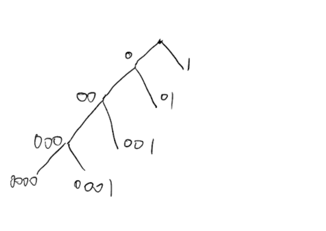
Figure 1. One possible pruned tree.

This theorem shows that the average length performance of prefix codes can be a representation of UDCs, because for any UDC, there exists a prefix code with the same codeword length, which has the best decoding performance.

Similarly, for certain RV \(X\), there exists a prefix code that achieves the entropy bound.

Note that it is not the proof of achievability, because for other RV \(X\), the bound cannot be directly achieved by coding a single \(X\).

Lemma 3.2.

There exists a \(D\)-ary prefix code \(\mathcal C\) such that \(\mathbb E[l(\mathcal C(X))]=H(X)\) iff \(\{p_i\}_{i\in[m]}\) are all \(D\)-adic.

Proof.

The “if” part is a derivation of construction from Theorem 3.1, and the “only if” part is from the equality condition of Theorem 2.2.

We give the proof based on the typical set.

1.4 Huffman and Shannon Fano’s Code

Next, we give a prefix-code construction with the minimum expected length (called optimal code) for any RV \(X\), known as the Huffman code.

Definition 4.1 (Huffman Code).

Let \(X:\Omega\to\mathcal X\) be an RV and \(D\geq2\) be a positive integer. We construct an RV \(X'\) with \(\mathcal X\subseteq\mathcal X'\) such that

\[\exists k\in\mathbb N_+,\qquad D+(k-1)(D-1)<\lvert\mathcal X\rvert \leq D+k(D-1)=\lvert\mathcal X'\rvert, \tag{1.15}\]

and

\[p_{X'}(x)= \begin{cases} p_X(x), & \forall x\in\mathcal X,\\ 0, & \forall x\in\mathcal X'\setminus\mathcal X. \end{cases} \tag{1.16}\]

The Huffman code \(\mathcal H:\mathcal X'\to[D]^{<\infty}\) is constructed by merging the \(D\) smallest probability masses together until the sum is \(1\). The codeword is the choice from root (\(p=1\)) to leaves (\(p=p_i\)).

We give some basic properties of optimal code.

Lemma 4.1.

Optimal code maps larger probabilities to shorter codewords.

Proof.

Suppose there are two probability masses \(p_i<p_j\) with optimal code lengths \(c_i<c_j\). We can exchange the two codewords to get a new prefix code, but

\[p_il_i+p_jl_j-p_il_j-p_jl_i =(p_j-p_i)(l_j-l_i)>0, \tag{1.17}\]

which contradicts the optimality.

Lemma 4.2.

There exists an optimal code \(\mathcal C\) in which the two smallest probabilities are siblings (have the same length and differ only in the last symbol).

Proof.

If not, we can code the smallest probability to its parent (note that it is longest and has no sibling) and reduce the length of the codeword by \(1\), which contradicts the optimality.

We further prove that the Huffman code is actually the optimal code.

Theorem 4.3.

Huffman code is optimal.

Proof.

Suppose an optimal code \(\mathcal C:\mathcal X\to[2]^{<\infty}\) and let \(\{p_i\}\) be the probabilities in descent order. For siblings \(p_{m-1}\) and \(p_m\), we merge them together and code the new probability by its parent. Then we get another prefix code \(\mathcal C^*\) with length

\[L(\mathcal C^*)=L(\mathcal C)-p_{m-1}-p_m.\]

We prove it is also optimal. Then we do this again until the probabilities are reduced to \(2\), and we merge them to get two codewords with length \(1\). This is exactly the procedure of Huffman code.

We turn our proof of achievability to the Huffman code’s upper bound.

Theorem 4.4 (Infimum of Huffman Code).

All expected lengths of Huffman code have an infimum:

\[\inf L(\mathcal H)=H(X)+1. \tag{1.18}\]

Proof.

Let \(X\) be an RV. Notice that Huffman code is the optimal code. As long as we construct a prefix code \(\mathcal C\) with expected length less than \(H(X)-1\), we can prove \(L(\mathcal H)<H(X)+1\). Consider a \(D\)-ary prefix code with codeword length \(l_i=\lceil-\log_Dp_i\rceil\). The existence of such a code \(\mathcal C\) is proved in Theorem 3.1, because \(\{l_i\}\) satisfies the Kraft inequality:

\[\sum_i\frac{p_i}{D} <\sum_iD^{-l_i} \leq\sum_i p_i=1. \tag{1.19}\]

Now we show the expected length:

\[L(\mathcal C)=\sum_i p_il_i \leq\sum_i p_i(-\log_Dp_i+1) =H(X)+1, \tag{1.20}\]

which shows that there exists a prefix code with expected length less than \(H(X)+1\).

To show that \(H(X)+1\) is the infimum, we prove that there exists a sequence of distributions \(\{P_k\}\) such that \(\lim_{k\to\infty}L(\mathcal H)\to H(X)+1\). This can be done by letting

\[P_k=\left\{1-\frac{D}{k},\frac{1}{k},\ldots,\frac{1}{k}\right\}. \tag{1.21}\]

For a \(D\)-ary Huffman code, the length of all possible codewords is always \(1\). As \(\lim_{k\to\infty}H(X)=0\),

\[\lim_{k\to\infty}L(\mathcal H) =1 =\lim_{k\to\infty}H(X)+1. \tag{1.22}\]

Thus, \(\forall\epsilon>0\), there exists \(k>D\) such that \(L(\mathcal H)>H(X)+1-\epsilon\), which finishes the proof.

Theorem 4.5 (Achievability of 0-error Data Compression II: By Huffman Code).

For any RV \(X\), Huffman code gives the entropy bound in the average sense, i.e.,

\[\forall X_1\overset{\mathrm{i.i.d.}}{\sim}X_2 \overset{\mathrm{i.i.d.}}{\sim}\cdots \overset{\mathrm{i.i.d.}}{\sim}X_n, \qquad \lim_{n\to\infty} \frac{\sum_{i=1}^nL(\mathcal H(X_i))}{n} =H(X). \tag{1.23}\]

Proof.

This is proved by the definition of prefix code (that the expanded code of Huffman code is also a Huffman code), and that

\[nH(X)=H(X_1,\ldots,X_n) \leq L(\mathcal H^*(X_1,\ldots,X_n)), \tag{1.24}\] \[=\sum_{i=1}^nL(\mathcal H(X_i)) <H(X_1,\ldots,X_n)+1 =nH(X)+1. \tag{1.25}\]

Definition 4.2 (Shannon Fano's Code).

Basically two questions. First, does it satisfy the Kraft inequality? Second question: how good is it?

Lemma 4.6 (Performance of Shannon Fano Code).

\[\mathbb E[l(\mathcal C(X))]\leq H(X)+1. \tag{1.26}\]

Proof.

\[\mathbb E[l(\mathcal C(X))] =\sum_{i\in[m]}p_il_i =\sum_{i\in[m]}p_i\lceil-\log p_i\rceil, \tag{1.27}\] \[\leq\sum_{i\in[m]}p_i(-\log p_i+1) =H(X)+1. \tag{1.28}\]

When samples \(n=1\), or relatively small, the code is not that good. But when \(n\) goes larger,

\[\frac{\mathbb E[l(\mathcal C(X))]}{n} \leq H(X)+\frac{1}{n} \to H(X),\qquad n\to\infty. \tag{1.29}\]

1.5 Mismatched Encoding

Consider Shannon Fano’s code designed for a PMF \(p\) while the true PMF of source \(X\) is \(q\).

Lemma 5.1 (Performance of mismatched).

\[\mathbb E[l(\mathcal C(X))] \in\left[D(q\mathbin{\Vert}p)+H(q),\ D(q\mathbin{\Vert}p)+H(q)+1\right]. \tag{1.30}\] \[\mathbb E[l(\mathcal C(X))] =\sum_xQ(x)\lceil-\log p(x)\rceil \tag{1.31}\] \[\leq D(q\mathbin{\Vert}p)+H(q)+1. \tag{1.32}\]

Meanwhile,

\[\mathbb E[l(\mathcal C(X))] =\sum_xQ(x)\lceil-\log p(x)\rceil \tag{1.33}\] \[\geq D(q\mathbin{\Vert}p)+H(q). \tag{1.34}\]

So here, KL divergence \(D(q\mathbin{\Vert}p)\) has a new physical meaning: penalty for using a code designed for \(p\) on \(q\).

1.6 Redundancy of Prefix Codes

Definition 6.1 (Related Definitions of Coding Tree).

Let \(X\sim\{p_1,\ldots,p_m\}\) be an RV and \(\mathcal C\) be a \(D\)-ary prefix code. Let \(G=(V,E)\) be the corresponding coding tree. Let \(I\) be the index set of all the internal nodes (including the root) in \(G\).

1. Reaching probability. For every \(k\in I\), the reaching probability \(q_k\) is the probability of reaching an internal node \(k\) during the decoding process.

2. Branching probability. For every \((k,j)=e\in E\), the branching probability \(\widetilde p_e\) is defined by the probability that the \(j\)-th branch of node \(k\) is taken during the decoding process.

3. Conditional branching probability. Once node \(k\in I\) is reached, the conditional branching distribution is defined by \(\{\widetilde p_e/q_k\}_{e\in\operatorname{Out}(k)}\).

4. Conditional entropy. The conditional entropy of node \(k\in I\) is defined by

   \[h_k=H_D\left(\left\{ \frac{\widetilde p_{(k,0)}}{q_k}, \frac{\widetilde p_{(k,1)}}{q_k}, \ldots, \frac{\widetilde p_{(k,D-1)}}{q_k} \right\}\right). \tag{1.35}\]

5. Local redundancy. The local redundancy of an internal node \(k\in I\) is \(r_k=q_k(1-h_k)\).

6. We say the node \(k\in I\) is balanced iff for every \((k,j)\in\operatorname{Out}(k)\), \(\widetilde p_{(k,j)}=q_k/D\).

From the above definitions, we can see that:

Lemma 6.1 (Basic Results in the Coding Tree).

1. Reaching probability is the sum of branches from which it is set out:

   \[q_k=\sum_{e\in\operatorname{Out}(k)}\widetilde p_e. \tag{1.36}\]

2. Local redundancy vanishes iff the node is balanced:

   \[\forall k\in I,\qquad r_k=0\Longleftrightarrow k\text{ is balanced}. \tag{1.37}\]

3. The entropy is defined by the structure of the code tree:

   \[H_D(X)=\sum_{k\in I}q_kh_k. \tag{1.38}\]

4. The expected length is defined by the sum of all internal reaching probabilities:

   \[L=\sum_{k\in I}q_k. \tag{1.39}\]

5. Local redundancy theorem:

   \[R=\sum_{k\in I}r_k. \tag{1.40}\]

Proof.

1. From the definition.

2. \(r_k=q_k(1-h_k)\), where \(h_k\leq1\) with equality iff the branch distribution is uniform, i.e., for every \((k,j)\in\operatorname{Out}(k)\), \(\widetilde p_{(k,j)}=q_k/D\).

3. Use induction on the number of internal nodes.

   Firstly, if there is an RV with only one internal node, i.e., the root, then by \(H_D(X)=h_0\) and \(q_0=1\) we get \(H_D(X)=q_0h_0\).

   Secondly, when it is true for every \(n\in\mathbb N_+\) internal nodes, then for RV \(X\) with \(n+1\) internal nodes, we merge the nodes with the longest codeword to its parent \(d\) and use the reaching probability \(q_d\) as the new leaf probability. Thus we construct a new RV \(X'\) with \(n\) internal nodes. We have

   \[\begin{aligned} H_D(X) &=\sum_{t\text{ is to a leaf}}\widetilde p_t\log_D\widetilde p_t\\ &=H_D(X') -\sum_{e\in\operatorname{Out}(d)}\widetilde p_e\log_D\widetilde p_e +q_d\log_Dq_d, \end{aligned} \tag{1.41}\] \[=H(X')+ \left( -\sum_{e\in\operatorname{Out}(d)}\widetilde p_e\log_D\widetilde p_e +\sum_{e\in\operatorname{Out}(d)}\widetilde p_e\log_Dq_d \right), \tag{1.42}\] \[=\sum_{k\in I\setminus\{d\}}q_kh_k -q_d\sum_{e\in\operatorname{Out}(d)} \frac{\widetilde p_e}{q_d} \log_D\frac{\widetilde p_e}{q_d} =\sum_{k\in I}q_kh_k. \tag{1.43}\]

4. Let \(k\in I\) and \(i\in\lvert\mathcal X\rvert\), and let \(a_{ki}\) be an indicator that takes the value \(1\) iff a leaf \(c_i\in\mathcal X\) is a descendant of internal node \(k\); otherwise \(a_{k,i}\) takes \(0\). We have

   \[l_i=\sum_{k\in I}a_{ki}, \qquad q_k=\sum_{i:c_i\in\mathcal X}a_{k,i}p(c_i). \tag{1.44}\] \[L=\sum_{i:c_i\in\mathcal X}p_il_i =\sum_{k\in I}\sum_{i:c_i\in\mathcal X}p_ia_{ki} =\sum_{k\in I}q_k. \tag{1.45}\]

5. From the definition of redundancy \(R=L-H_D(X)\).

The theorem of entropy bound (Theorem 1.2) is then expressed by:

Theorem 6.2 (Capacity of 0-error Data Compression).

The redundancy of any prefix code \(R=L-H(X)\geq0\), with equality iff all the internal nodes are balanced.

Proof.

Omitted.

This expression gives us more details that every internal node must be balanced (where the former only requires the probabilities of terminal nodes). An intuitive explanation is that the entropy bound resylts from the fact that a \(D\)-ary symbol carries at most \(D\)-it of information. The achievability of balanced nodes guarantees that, as long as an codeword is not completed, the next symbol has must carries o 1 \(D\)-it of information, which meets our intuition that entropy is a measure of information on its expected coded length.

Comments