CATALOG

• Non-Bayesian Detection problem: Neyman-Pearson
• Asymptotic NP Detector
• Bayes Hypothesis Testing
• (P_{e}) and Total Variation
• Bayes Estimation Theory

In data compression, consider \(X_{[n]}\stackrel{i.i.d}{\sim}Ber(p)\), then they can be compressed into \(nh_{b}(p)\) bits.

Non-Bayesian Detection problem: Neyman-Pearson

Suppose one wants to detect whether two of the scenarios is true: (\(H_{1}\)): \(X\sim P_{0}\), or (\(H_{2}\)): \(X\sim P_{1}\). One observe \(x^{n}\) generated i.i.d. with \(X\). A detector is a function \(f: \mathcal{X}^{n}\to \{0,1\}\)

Definition 1.1 (Decision Region).

If \(x_{(n)}\in A_{n}\) then detect \(X\sim P_{0}\), or not present
If \(x_{(n)}\in A_{n}^{c}\) then detect \(X\sim P_{1}\), or present. \(A_{n}\) is called rejection region.

Definition 1.2 (2 kinds of errors).

\[\begin{align} \alpha = P_{0}(A_{n}^{c}) \text{ false-alarm prob.}\\ \beta = P_{1}(A_{n}) \quad \text{mis-detection prob} \end{align}\]

One key question is to minimize \(\beta\) s.t. \(\alpha \leq \epsilon\) (fixed), and how to design the optimal decision region. This is called a non-Bayes estimation. (Note: Bayes estimation is when the prior probability of parameters to be estimated is known.)

Theorem 1.1 (Neyman Pearson Theorem).

Let \(T>0\), \(A_{n}(T)\) is the decosion region with LRT with threshold \(T\), i.e.,

\[\begin{align} A_{n}(T) =\{x^{n}: \frac{P_{0}(x^{n})}{P_{1}(x^{n})}>T\} \end{align}\]

Let \(\alpha ^{\star}(T) = P_{0}(A_{n}^{C}(T))\), and \(\beta ^{\star}(T) = P_{1}(A_{n}(T))\), then if \(\alpha, \beta\) is the FA and MD prob., \(\alpha \leq \alpha ^{\star}\Rightarrow \beta \leq \beta ^{\star}\)

(Note: We call \(A_{n}(T)\) the NP region.) (Note: This works for any finite \(n\).)

Proof.

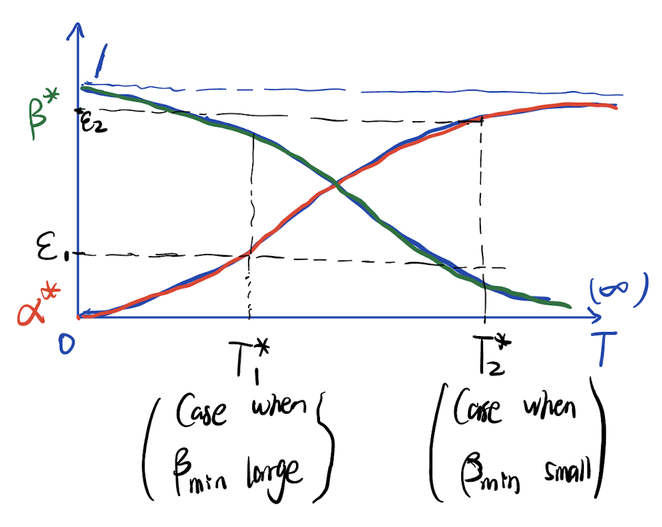Performance of NP Detection as FA and MD with \(T\)

Suppose \(A_{n}^{T}\) is the NP region and \(B_{n}\) is any other region. Let

\[\begin{align} \phi_{A}(x^{n}) = \mathbf{1}_{\{x^{n}\in A_{n}\}},\quad \phi_{B}(x^{n}) = \mathbf{1}_{\{x^{n}\in B_{n}\}} \end{align}\]

we have \(\forall x^{n}\in\mathcal{X}^{n}\),

\[\begin{align} 0\leq \left( \phi_{A}(x^{n}) - \phi_{B}(x^{n}) \right) \left( P_{0}(x^{n}) - TP_{1}(x^{n}) \right) \end{align}\]

because it both holds when \(x^{n}\in A_{n}\) and \(x^{n}\in A_{n}^{C}\). Then

\[\begin{align} 0\leq & \sum_{x^{n}} \left( \phi_{A}(x^{n}) - \phi_{B}(x^{n}) \right) \left( P_{0}(x^{n}) - TP_{1}(x^{n}) \right) \\ =& P_{0}(A_{n}) - P_{1}(B_{n}) - T(P_{1}(A_{n}) - P_{1}(B_{n}))\\ = & (\alpha - \alpha ^{\star}) + T(\beta - \beta ^{\star}) \end{align}\]

which is a Lipshitz condition saying that \(\alpha \leq \alpha ^{\star}\Rightarrow \beta \leq \beta ^{\star}\).

Asymptotic NP Detector

Definition 2.1 (Asymptotic NP Detection).

A decision region with parameters \(n\), i.e., \(A_{n}\subseteq \mathcal{X}^{n}\). A non-negative \(D\geq 0\) is said to be achievable if \(\forall \epsilon>0\), there exists a detector \(\{f_{n}\}_{n\in\mathbb{N}}\) and \(N(\epsilon)\) s.t. \(\forall n\geq N(\epsilon)\), \(\alpha_{n} = P_{0}(A_{n}^{C})<\epsilon\), and \(\frac{\log \beta_{n}}{n}\leq - D + \epsilon\).

(Note: Alternatively, \(D\) is said to be achievable if \(\forall \epsilon>0\), there exists a sequence of detector \(\{f_{n}\}\) s.t. \(\alpha_{n}\to 0\) and \(-\frac{\log \beta_{n}}{n}\to D\)) .

Definition 2.2 (Capacity).

\[\begin{align} D^{\star} = \sup \{D: D\text{ is achievable}\} \end{align}\]

Theorem 2.1 (Capacity of NP Detection with zero FA, Stein's Lemma).

\[\begin{align} D^{\star} = D(P_{0}\Vert P_{1}) \end{align}\]

Definition 2.3 (Functional Typical).

Let \(f:\mathcal{X}\to [1:n]\), and \(D(X) = \mathbb{E}[f(X)]\). For a sequence \(x^{n}\) generated from \(n\) i.i.d. RV \(X_{i}\sim X\), \(x^{n}\) is said to be \(f\)-typical iff

\[\begin{align} x^{n}\in \mathcal{T}_{f,\epsilon}^{n}\iff \left\vert \frac{\sum_{n} f(x)}{n} - \mathbb{E}[f(X)] \right\vert \leq \epsilon \end{align}\]

Example 2.1.

1. \(f(x) =- \log p(x)\), then it becomes the Week typical set.
   
2. \(f(x) = \log \frac{P(x)}{Q(x)}\), then the set becomes the relative typical set \(\mathcal{T}_{\epsilon}^{n}(P_{1}\Vert P_{2})\)

Bayes Hypothesis Testing

In this setting the prior \(\pi_{0}, \pi_{1}\) is given. The problem is

\[\begin{align} \min_{A_{n}}\pi_{0}\alpha + \pi_{1}\beta \end{align}\]

An important observation is that the boundary of \(A_{n}\), i.e., the region to make \(H_{1}\), is with type.

Theorem 3.1 (Sanov's Theorem).

Let \(X_{(n)}\) be \(n\) i.i.d. DRV. \(E\) be a collection of all types in of \(x^{n}\). We have

\[\begin{align} (n + 1)^{-\vert \mathcal{X}\vert }2^{- nD(Q^{*}\Vert P)}\leq \sum_{Q\in E} P(\mathcal{A}_{Q}^{n})\leq (n + 1)^{\vert \mathcal{X}\vert }2^{- nD(Q^{*}\Vert P)} \end{align}\]

where \(Q^{*} = \arg\min_{Q\in E}D(Q\Vert P)\).

To solve the minimum problem, 5 steps are there to prove the optimal \(\alpha,\beta\) in the Bayes testing

STEP 1: Using Sanov’s Theorem implies that \(\sum_{Q\in E} P(\mathcal{A}_{Q}^{n})\stackrel{\sim}{\sim} 2^{- nD(Q^{*}\Vert P)}\).

STEP 2: NP-test

\[\begin{align} A_{n}(T) =& \left\{ x^{n}:\frac{1}{n}\log\frac{P_{1}^{n}(x^{n})}{P_{2}^{n}(x^{n})}\geq \frac{1}{n}\log T \right\} \\ =& \left\{ x^{n}:\sum_{a\in \mathcal{X}}\frac{N(a\vert x^{n})}{n} \log \frac{P_{1}(a)}{P_{2}(a)}\geq \frac{1}{n}\log T \right\} \\ \end{align}\]

Notice

\[\begin{align} \sum_{a\in \mathcal{X}}\frac{N(a\vert x^{n})}{n} \log \frac{P_{0}(a)}{P_{1}(a)} =& \sum_{a\in \mathcal{X}}P(a)\log \frac{P_{0}(a)}{P_{1}(a)}\\ =& - D(P\Vert P_{0}) + D(P\Vert P_{1}) \end{align}\]

so NP test is \(A_{n}(T) = \left\{ x^{n}: - D(P\Vert P_{0}) + D(P\Vert P_{1})\geq \frac{1}{n}\log T \right\}\)

STEP 3:

\[\begin{align} \alpha_{n} =& P_{0}^{n}(A_{n}^{C})\stackrel{R}{\sim} -D(P_{0}^{\star}\Vert P_{0})\\ \beta_{n} =& P_{1}^{n}(A_{n}^{C})\stackrel{R}{\sim} - D(P_{1}^{\star}\Vert P_{1}) \end{align}\]

where

\[\begin{align} P_{0}^{\star}\in \arg\min_{p}D(p\Vert P_{0}) \end{align}\]

STEP 4: Optimization. (Remove the constraint that \(P\) is a type of solution \(n\). The minimized \(P\) is losser but still a UB).

\[\begin{align} \min & D(P\Vert P_{0})\\ s.t. & D(P\Vert P_{1}) - D(P\Vert P_{0})\leq \frac{1}{n}\log T\\ & \sum_{a}P(a) = 1\\ & P(a)>0 \end{align}\]

We use Lagrange Multiplier here.

\[\begin{align} J = D(P\Vert P_{0}) + v\sum_{a}P(a) + \lambda \sum_{a}P(a)\log\frac{P_{0}(a)}{P_{1}(a)} + \sum_{a} Q(a)P(a) \end{align}\] \[\begin{align} & \frac{\partial J}{\partial P(a)} = 0\\ \Rightarrow& \log \frac{P(a)}{P_{0}(a)} + \log_{2} e + v + \lambda \log \frac{P_{0}(a)}{P_{1}(a)} + Q(a) = 0\\ \Rightarrow & P(a) = 2^{- v - Q(a) - \log_{2} e}\frac{P_{1}^{\lambda}(a)}{P_{0}^{\lambda- 1}(a)} \end{align}\]

notice from the formula that constraint \(P(a)\geq 0\) is not active, i.e., \(Q(a) = 0\). Therefore, for active constraint \(\sum_{a}P(a) = 1\), \(v\) is chosen accordingly by

\[\begin{align} P(a) =\frac{P_{1}^{\lambda}(a)P_{0}^{1 - \lambda}(a)}{\sum_{a}P_{1}^{\lambda}(a)P_{0}^{1 - \lambda}(a) } \end{align}\]

Due to the structure of the problem, the constraint \(D(P\Vert P_{1}) - D(P\Vert P_{0})\geq \frac{1}{n}\log T\) is active and satified with equality, i.e., choose \(\lambda\) s.t.

\[\begin{align} D(P\Vert P_{1}) - D(P\Vert P_{0}) = \frac{1}{n}\log T \end{align}\]

Optimize \(P_{1}^{\star}\) is similar:

\[\begin{align} \min_{P}& D(P\Vert P_{1})\\ s.t. & D(P\Vert P_{1}) - D(P\Vert P_{0})\geq \frac{1}{n}\log T & \sum_{a}P(a) = 1 & P(a)\geq 0 \end{align}\]

using similar steps,

\[\begin{align} P(a) =\frac{P_{0}^{\lambda}(a)P_{1}^{1 - \lambda}(a)}{\sum_{a}P_{0}^{\lambda}(a)P_{1}^{1 - \lambda}(a) } \end{align}\]

where \(\lambda\) satisfying \(D(P\Vert P_{1}) - D(P\Vert P_{0}) = \frac{1}{n}\log T\). By letting \(\gamma = 1 - \lambda\), we notice that the \(P_{1}^{\star} = P_{2}^{\star} = P^{\star}\) because \(\lambda,\gamma\) in the two formula follows the same constraint, and the two distribution follows the same formula w.r.p. \(\lambda\) and \(\gamma\).

STEP 5: the answer

\[\begin{align} &\pi_{0}2^{- nD(P^{\star}\Vert P_{0})} + \pi_{1}2^{- nD(P^{\star}\Vert P_{1})}\\ \leq & 2^{- n\min\{D(P^{\star}\Vert P_{0}),D(P^{\star}\Vert P_{1}) \}} \end{align}\]

optimality is achieved when \(D(P^{\star}\Vert P_{0}) = D(P^{\star}\Vert P_{1})\), i.e., \(\alpha \stackrel{R}{\sim} -D(P^{\star}\Vert P_{0})\) and \(\beta \stackrel{R}{\sim} -D(P^{\star}\Vert P_{1})\) has the same rate. Then we can solve \(\lambda\):

\[\begin{align} \lambda \end{align}\]

so,

\(P_{e}\) and Total Variation

For distribution \(P,Q\), \(TV = \frac{1}{2}\Vert P - Q\Vert\).

A trivial Bayes testing where \(n = 1\), \(\pi_{0} = \pi_{1} = \frac{1}{2}\), then \(A_{1} =\{x:\frac{P_{1}(x)}{P_{0}(x)}> 1\}\), and

\[\begin{align} P_{e} = \frac{1}{2} - \frac{1}{2}TV(P_{1}P_{0}) \end{align}\]

generally,

\[\begin{align} TV(P_{0},P_{1}) =& \frac{1}{2}\sum_{x^{n}\in A_{n}}\vert P_{1}(x^{n}) - P_{0}(x^{n})\vert + \frac{1}{2}\sum_{x^{n}\in A_{n}^{C}}\vert P_{1}(x^{n}) - P_{0}(x^{n})\vert \\ =& \frac{1}{2}\sum_{x^{n}\in A_{n}}(P_{1}(x^{n}) - P_{0}(x^{n})) + \frac{1}{2}\sum_{x^{n}\in A_{n}^{C}}(P_{0}(x^{n}) - P_{1}(x^{n}))\\ =&\frac{1}{2}\left( P_{1}(A_{n}) - P_{0}(A_{n}) + P_{0}(A_{n}^{C}) - P_{1}(A_{n}^{C}) \right) \\ =& P_{0}(A_{n}) - P_{1}(A_{n}) \end{align}\]

Theorem 4.1 (Tensorization).

1. N-P Testing Rate:

\[\begin{align} D(P_{0}\times P_{0}\Vert P_{1}\times P_{1}) = D(P_{0}\Vert P_{1}) + D(P_{0}\Vert P_{1}) \end{align}\]

1. Bayes Testing Rate:

\[\begin{align} C(P_{0}\times P_{0}\Vert P_{1}\times P_{1}) = C(P_{0}\Vert P_{1}) + C(P_{0}\Vert P_{1}) \end{align}\]

1. TV: Cannot Tensorize:

\[\begin{align} TV(P_{0}\times P_{0}\Vert P_{1}\times P_{1}) =\Vert P_{0}\times P_{0} -P_{1}\times P_{1}\Vert \neq \Vert P_{0} -P_{1}\Vert + \Vert P_{0} -P_{1}\Vert \end{align}\] \[\begin{align} \Vert P_{0}^{n} -P_{1}^{n}\Vert \sim 2^{-nC(P_{1}\Vert P_{2})} \end{align}\]

Bayes Estimation Theory

Let \(X_{(n)}\) be i.i.d. observation with PMF \(P_{X;\theta}\) with unknown parameter \(\theta\). The objective is to estimate \(\theta\) as a function of \(x^{n}\) as \(\hat{\theta} = T(X_{(n)})\). We call \(\hat{\theta}\) the estimation and \(T\) the estimator.

Definition 5.1 (Performance of Estimator).

We say \(T\) or \(\hat{\theta}\) is

1. Unbiased, iff \(\mathbb{E}[\hat{\theta}]= \mathbb{E}[T(X_{(n)})]= 0\).

2. Minimal Variance, if \(\forall T^{\prime}\), \(Var(T(X_{(n)}))\leq Var(T^{\prime}(X_{(n)}))\).

Any estimator which is unbiased and has minimal variance is called Min variance Unbiased Estimator (MVUE).

Theorem 5.1 (Cramer-Rao Bound).

Any unbiased estimator \(T:\mathcal{X}^{n}\to \Theta\) has bound

\[\begin{align} Var(T(X_{(n)}))\geq \frac{1}{nJ(\theta)} \end{align}\]

where \(J(\theta)\) is called the Fisher Information and

\[\begin{align} J(\theta) = Var\left[ \frac{ \partial }{ \partial \theta }\ln P_{X;\theta}(X) \right] \end{align}\]

(Note: Larger Fisher Information, the smaller the minimum variance will be, the better the MVUE performs.)

Proof.

\[\begin{align} \mathbb{E}\left[ \frac{ \partial }{ \partial \theta }\log P_{X;\theta}(X) \right] =& \sum_{x}P_{X;\theta}(x)\frac{ \partial }{ \partial \theta } \log P_{X;\theta}(x)\\ =& \sum_{x}\frac{ \partial }{ \partial \theta } P_{X;\theta}(x)\\ =& \frac{ \partial }{ \partial \theta }\left[ \sum_{x}P_{X;\theta}(x) \right] \\ =& 0 \end{align}\]

therefore,

\[\begin{align} J(\theta) =Var\left[ \frac{ \partial }{ \partial \theta }\ln P_{X;\theta}(X) \right] = \mathbb{E}\left[ \left(\frac{ \partial }{ \partial \theta }\ln P_{X;\theta}(X) \right)^{2} \right] \end{align}\]

According to Cauchy-Schwartz Inequality (\(Cov(X,Y)^{2}\leq Var(X)Var(Y)\)),

\[\begin{align} \sum_{x}T(x^{n}) \end{align}\]

Example 5.1.

Let i.i.d. \(X_{(n)}\sim Ber(\theta)\). Testing the performance of \(T(X_{(n)}) = \bar{X} = \frac{1}{n}\sum X_{(n)}\).

First, \(\mathbb{E}[T]= \theta\), i.e., Unbiased.

Second, \(Var(T) = \frac{1}{n}Var(X) = \frac{\theta(1 - \theta)}{n}\).

Third, \(\frac{ \partial }{ \partial \theta }\log P_{X;\theta}(X) = \frac{1}{\theta}\) w.p. \(\theta\) and \(\frac{1}{1 - \theta}\) w.p. \((1 - \theta)\). So

\[\begin{align} J(\theta) = Var\left[ \frac{ \partial }{ \partial \theta }\log P_{X;\theta}(X) \right]= \mathbb{E}\left[ \left( \frac{ \partial }{ \partial \theta }\log P_{X;\theta}(X) \right)^{2} \right] =\frac{1}{\theta(1 - \theta)} \end{align}\]

This estimation is best because \(\frac{1}{nJ(\theta)} = \frac{\theta(1 - \theta)}{n}\).

Comments