CATALOG
We aim to develop a theory which establishes a one-to-one correspondence between Shannon’s information measures and set theory in full generality. Moreover, for finite RVs, Shannon’s information measures can be visualized by mean of information digram.
Preliminaries of Measure Theory
Definition 1.1.
(Atoms of Field):
Let \(n\in \mathbb{N}_+\) and \(\mathcal{F}_n\) be a finite field generated by \(n\) sets \(\tilde{X}_1,\cdots \tilde{X}_n\), i.e., \(\mathcal{F}_n\) is the collection of sets operated by set operations (union, intersection, complement) on \(\tilde{X}_1,\cdots \tilde{X}_n\). Then we call the atoms of \(\mathcal{F}_n\) are the sets of the form \(\bigcap_{i=1}^{n}Y_i\), where \(Y_i\) is either \(\tilde{X}_i\) or \(\tilde{X}^c_i\).
Lemma 1.1.
\(\vert \mathcal{F}_n\vert =2^{2^n}\) whereas only \(2^n\) atoms whose union is the complete set \(\Omega\) and intersection is the empty set \(\emptyset\).
In the context, we always ignore the atoms of \(\mathcal{F}_n\) which is empty.
Definition 1.2.
(Signed Measure):
A real function \(\mu: \mathcal{F}_n\to \mathbb{R}\) is called a signed measure iff \(\mu\) is non-negativity and countably union-addictive, i.e.,
\[\begin{align} \forall A\in\mathcal{F}_n,& \quad \mu(A)\geq 0\\ \forall A, B\in\mathcal{F}_n, A\cap B=\emptyset,&\quad \mu(A\cup B)=\mu(A)+\mu(B) \end{align}\]
(Note: From the definition we know that there may be more than one signed measure on a given field \(\mathcal{F}_n\).) (Note: We call \(\mu\) a signed measure rather than a measure, for that \(\mu\) may give a negative value on some sets.)
Lemma 1.2.
- \[\mu(\emptyset)=0\]
- \(\forall A,B\in \mathcal{F}, A\subseteq B\to \mu(A)\leq \mu(B)\).
- A signed measure \(\mu\) on \(\mathcal{F}_n\) is completely specified by its values on atoms:
\[\begin{align} \forall A\in \mathcal{F}, \mu(A)=\sum_{i=1}^{2^n}a_i\mu(A_i) \end{align}\]
where \(a_i\) takes value in \(0\) or \(1\) while \(A_i\) is the atoms of \(\mathcal{F}_n\).
Construction of I-Measure
We take \(\mathcal{F}_2\) generated by \(\tilde{X}_1,\tilde{X} _2\) with \(\Omega:=\bigcup \mathcal{F}_2=\tilde{X}_1\cup\tilde{X} _2\) as an example. So there are only 3 nonempty atoms. Let \(\tilde{X}_1,\tilde{X} _2\) be sets corresponding to \(X_1\) and \(X_2\) resp. We aim to give a one-to -one correspondence between Shannon’s measure and the signed measure \(\mu^*\) on \(\mathcal{F}_2\), in the manner of the following listed atoms:
\[\begin{align} \mu^*(\tilde{X}_1-\tilde{X}_2)=&H(X_1\vert X_2)\\ \mu^*(\tilde{X}_2-\tilde{X}_1)=&H(X_2\vert X_1)\\ \mu^*(\tilde{X}_1\cap\tilde{X} _2)=&I(X_1;X_2) \end{align}\]From the definition of signed measure (Signed Measure),
\[\begin{align} \mu^*(\tilde{X}_1)=&\mu^*(\tilde{X}_1\cap\tilde{X} _2)+\mu^*(\tilde{X}_1-\tilde{X}_2)=I(X_1;X_2)+H(X_1\vert X_2)=H(X_1)\\ \mu^*(\tilde{X}_2)=&\mu^*(\tilde{X}_1\cap\tilde{X} _2)+\mu^*(\tilde{X}_2-\tilde{X}_1)=I(X_1;X_2)+H(X_2\vert X_1)=H(X_2)\\ \mu^*(\tilde{X}_1\cup\tilde{X}_2)=&\mu^*(\tilde{X}_1)+\mu^*(\tilde{X}_2-\tilde{X}_1)=H(X_1)+H(X_2\vert X_1)=H(X_1,X_2) \end{align}\]By observing each of these equations, the following left side and right side correspond to each other via the substitution of symbols:
\[\begin{align} H/I\leftrightarrow & \mu^* \qquad ,\leftrightarrow \cup\\ ;\leftrightarrow & \cap\qquad \vert \leftrightarrow - \end{align}\](Note: we make no distinction between the symbols \(H\) and \(I\) in this substitution. ) We need to remark that the value of \(\mu^*(\tilde{X}_1^c\cap \tilde{X}_2^c)\) has no apparent information-theoretic meaning, so we empty the set to vanish the signed measure to make sure \(\mu^*\) is completely specified by all Shannon’s information measures involving the RVs \(X_1\) and \(X_2\).
We then come to the general cases with \(n\geq 2\) RVs \(X_1,\cdots,X_n\). Similar to 2 RVs,
\[\begin{align} \Omega :=\bigcup \mathcal{F}_2=\bigcup_{i=1}^{n}\tilde{X}_i \end{align}\]so the only empty atom of \(\mathcal{F}_n\) is \(A_0=\bigcap_{i=1}^{n}\tilde{X}_i^c\). Let \(\mathcal{A}\) be the set of all nonempty atoms of \(\mathcal{F}_n\), we have:
Lemma 2.1.
(Inclusion-Exclusion Formula):
For a set-additive function \(\mu\),
\[\begin{align} \mu(\bigcap_{i=1}^{n}A_i-B)=\sum_{i=1}^{n}\mu(A_i-B)-\sum_{1\leq i\leq j\leq n}\mu(A_i\cup A_j-B)+\cdots+(-1)^{n+1}\mu(\bigcup_{i=1}^{n}A_i-B) \end{align}\]
Proof.
By induction. See details in probability analysis textbooks.
Theorem 2.2.
(Measure Specifying Theorem):
Let
\[\begin{align} \mathcal{B}=\{\bigcup_{k\in G}\tilde{X}_k: G\subseteq [n]\} \end{align}\]
then any signed measure \(\mu\) on \(\mathcal{F}_n\) is linearly specified by its values on the sets in \(\mathcal{B}\).
(Note: We later see that although \(\mu\) is not unique, there are only one signed measure \(\mu^*\) which is consistent with all Shannon’s measures.)
Proof.
From (Measure Specifying Theorem B) we know that any signed measure \(\mu\) on \(\mathcal{F}_n\) is linearly specified by its values on atoms, i.e., the sets in \(\mathcal{A}\). We now prove that there is a linear and invertible transformation between \(\{\mu(A):A\in\mathcal{A}\}\) and \(\{\mu(B):B\in\mathcal{B}\}\). Apparently, \(\vert \mathcal{A}\vert =\vert \mathcal{B}\vert =2^n-1\).
On the one hand, \(\forall B\in\mathcal{B}\subseteq \mathcal{F}_n\), so all sets in \(\mathcal{B}\) can be expressed uniquely as the union of some nonempty atoms in \(\mathcal{A}\). Let \(\vec{u},\vec{h}\) be two \(2^n-1\)-dimension vectors of \(\{\mu(A):A\in\mathcal{A}\}\) and \(\{\mu(B):B\in\mathcal{B}\}\), we then have
\[\begin{align} \bar{\exists} \mathbf{C}_n\in \{0,1\}^{n\times n},\quad \vec{h}=\mathbf{C}_n\vec{u} \end{align}\]One the other hand, a nonempty atom of \(\mathcal{F}_n\) has the form \(\bigcap_{i=1}^{n}Y_i\) with \(Y_i\) is either \(\tilde{X}_i\) or \(\tilde{X}_i^c\) with at least one \(i\in [n]\) such that \(Y_i=\tilde{X}_i\). So for any atom of \(\mathcal{F}_n\), we can write as
\[\begin{align} \bigcap_{i\in [n]: Y_i=\tilde{X}_i}\tilde{X}_i-\left(\bigcap_{j\in [n]: Y_j=\tilde{X}_j^c}\tilde{X}_j\right) \end{align}\]Note that the first part (intersection part) is non-empty. We can use the Inclusion-Exclusion Formula in (Inclusion-Exclusion Formula) and
\[\begin{align} \mu(A-B)=\mu(A\cup B)-\mu(B) \end{align}\]to prove that \(\forall A\in\mathcal{A}\), \(\mu(A)\) can be expressed as a linear combination of \(\mu(B)\) for \(B\in \mathcal{B}\). Consequently, there exists a \(k\times k\) matrix \(\mathbf{D}_n\) that
\[\begin{align} \vec{u}=\mathbf{D}_n\vec{h}=(\mathbf{D}_n\mathbf{C}_n)\vec{u} \end{align}\]In fact, \(\mathbf{D}_n\) is unique as \(\mathbf{C}_n\) is unique. So \(\{\mu(A):A\in\mathcal{A}\}\) is uniquely determined once \(\{\mu(B):B\in\mathcal{B}\}\) is specified. Hence, a signed measure \(\mu\) on \(\mathcal{F}_n\) is completely specified by \(\{\mu(B):B\in\mathcal{B}\}\), which can be valued at any set of nonnegative real numbers.
According to Measure Specifying Theorem (Measure Specifying Theorem B), we can construct a signed measure \(\mu^*\) which is consistent with Shannon’s Measures.
Theorem 2.3 (Constructions of I Measure).
The signed measure \(\mu^*\) generated by:
\[\begin{align} \forall \emptyset\neq G\in[n],\quad \mu^*(\bigcup_{k\in[n],k\in G}\tilde{X}_k)=H(X_{(G)}) \end{align}\]
is the unique signed measure on \(\mathcal{F}_n\) which is consistent with all Shannon’s Measures.
Proof.
\(\forall G,G',G''\subseteq [n]\), we have
\[\begin{align} &\mu^*\left(\left(\bigcup_{i\in[n],i\in G}\tilde{X}_i\right)\cap \left(\bigcup_{j\in[n],ji\in G'}\tilde{X}_j\right)-\left(\bigcup_{k\in[n],k\in G''}\tilde{X}_k\right)\right)\\ =& \mu^*\left(\bigcup_{i\in[n],i\in G\cup G''}\tilde{X}_i\right)+\mu^* \left(\bigcup_{j\in[n],ji\in G'\cap G''}\tilde{X}_j\right)-\mu^*\left(\bigcup_{k\in[n],k\in G\cap G'\cap G''}\tilde{X}_k\right)-\mu^*\left(\bigcup_{k\in[n],k\in G''}\tilde{X}_k\right)\\ =&H(X_{(G\cap G'')})+H(X_{(G'\cap G'')})-H(X_{(G\cap G'\cap G'')})-H(X_{(G'')})\\ =& I(X_{(G)};X_{(G')}\vert X_{(G'')}) \end{align}\]as all Shannon’s information measures can be expressed with conditional mutual information, \(\mu^*\) is then consistent with all Shannon’s information measures.
For the uniqueness, any signed measure \(\mu\) which is consistent with all Shannon’s measures has to satisfy (Constructions of I Measure), which is in fact the definition of \(\mu^*\) (because the values of the definition on \(\mu^*\) uniquely specifies a signed measure, by (Measure Specifying Theorem B)). Therefore, \(\mu^*\) is the unique signed measure on \(\mathcal{F}_n\) which is consistent with all Shannon’s information measures.
In the following relation, we focus on the \(\mu^*\) and show that \(\mu^*\) can take negative values for \(n\geq 3\). (Note: This indicates that not all I measure on atoms \(A\in\mathcal{A}\) is Shannon’s information measure) We exemplify the case when \(n=3\).
Example 2.1.
(\(\mu^*\) takes negative value for \(n= 3\)):
The 7 nonempty atoms of \(\mathcal{F}_3\) are:
where the values of \(\mu^*\) on 6 of them are Shannon’s information measure:
\[\begin{align} \mu^* (\tilde{X}_i-(\tilde{X}_j\cup \tilde{X}_k))=H(X_i\vert X_j,X_k)\\ \mu^*(\tilde{X}_i\cap \tilde{X}_j-\tilde{X}_k)=I(X_i;X_j\vert X_k) \end{align}\]while \(\mu^*(\tilde{X}_1\cap \tilde{X}_2\cap \tilde{X}_3)\) does not correspond to a Shannon’s information measure. Let \(X_1,X_2\) be i.i.d. u.d. in \(\{0,1\}\) and \(X_3=X_1 \oplus X_2\). Then we have
\[\begin{align} H(X_i)=1,\quad X(X_i,X_j)=2, \quad H(X_1,X_2,X_3)=2,\quad I(X_i;X_j)=0 \end{align}\]Therefore,
\[\begin{align} &\mu^*(\tilde{X}_1\cap \tilde{X}_2\cap \tilde{X}_3)\\ =& \mu^*(\tilde{X}_1\cup \tilde{X}_2\cup\tilde{X}_3)-\mu^*(X_1\cup \tilde{X}_2)-\mu^*(X_1\cup \tilde{X}_3)-\mu^*(\tilde{X}_2\cup\tilde{X}_3)+\mu^*( \tilde{X}_1)+\mu^*(\tilde{X}_2)+\mu^*(\tilde{X}_3)\\ =& H(X_1,X_2,X_3)-H(X_1,X_2)-H(X_1,X_3)-H(X_2,X_3)+H(X_1)+H(X_2)+H(X_3)\\ =& 2-2-2-2+1+1+1=-1 \end{align}\]Motivated by the substitution of symbols, we will write \(\mu^*(\tilde{X}_1\cap \tilde{X}_2\cap \tilde{X}_3)\) as \(I(X_1;X_2;X_3)\).
Definition 2.1.
(McGill’s mutual information, Lautum Information):
In general, for \(G_1,\cdots, G_m, F\in [n]\), we write \(\mu^*(\bigcap_{i\in G_1\cap G_2\cap\cdots\cap G_m-F}\tilde{X}_{i})\) as \(I(X_{G_1};X_{G_2};\cdots;X_{G_m}\vert X_F)\) and refer to it as the mutual information between \(X_{G_1},X_{G_2},\cdots,X_{G_m}\) conditioning on \(X_F\).
Lemma 2.4.
\[\begin{align} I(X_{G_1};X_{G_2};\cdots;X_{G_m};X_F)=I(X_{G_1};X_{G_2};\cdots;X_{G_m})-I(X_{G_1};X_{G_2};\cdots;X_{G_m}\vert X_F) \end{align}\](Note: We think of \(I\) as a functional symbol which takes \(X_G\), the set of RVs, into calculation. It denotes the function whose domain is the vector \(X_{(G)}\).)We need to pay extra attention that unlike entropy, the mutual information between RVs can be increased by conditioning on a third RV.
Lemma 2.5.
\(\forall n\in \mathbb{N}_+, n\geq 2,\) we have:
\[\begin{align} I(X_1;\cdots ;X_n)=E\log \frac{\prod_{i\in [n]_e}\left(\prod_{\mathcal{E}_i\subseteq [n],\vert \mathcal{E}_i\vert =i}p(X_{\mathcal{E}_i})\right)}{\prod_{i\in [n]_o}\left(\prod_{\mathcal{E}_i\subseteq [n],\vert \mathcal{E}_i\vert =i}p(X_{\mathcal{E}_i})\right)} \end{align}\]where \([n]_e\) and \([n]_o\) is the even (odd) elements of \([n]\).
Lemma 2.6.
\[\begin{align} -\min \{I(X;Y\vert Z),I(X;Z\vert Y),I(Y;Z\vert X)\}\leq I(X;Y;Z)\leq \min \{I(X;Y),I(X;Z),I(Y;Z)\}. \end{align}\]Information Diagrams
Definition 3.1.
(Information Digram):
Let \(X_1,\cdots, X_n\) be \(n\in\mathbb{N}\) RVs. The Venn digram w.r.t. sets \(\tilde{X}_i\) with \(\mu^*(\tilde{X}_i)=H(X_i)\) is called the information digram of \(X_1,\cdots,X_n\).
We do not display the atom \(A\in \mathcal{F}_n\) where \(\mu^*(A)=0\) in the information digram becacuse \(A\) does not contribute to \(\mu^*(B)\) for any set \(B\in\mathcal{F}_n\) and \(A\subseteq B\).
Apparently, the relations between all Shannon’s information measures and conditional mutual informations can be represented in the information digram. For an instance, the \(I\)-measure for 3 RVs \(X_1,X_2,X_3\) can be listed in a plane. For \(n\geq 4\), it is not possible to display an information diagram perfectly in two dimensions. In general, an information diagram for \(n\) random variables needs \(n-1\) dimensions to be displayed perfectly.
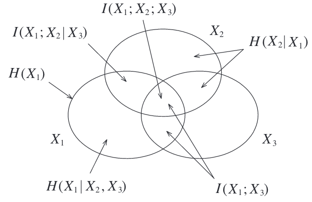
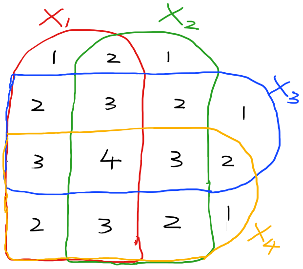
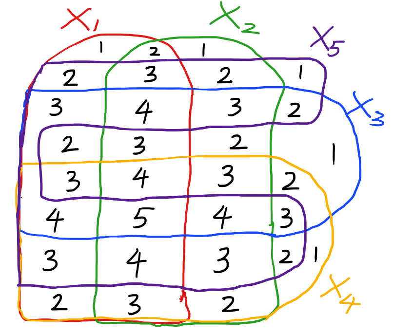 Information diagrams for (\(n=3,4,5\)) RVs
Although some atoms may be vanished in the information digram in certain structures (e.g., Markov constraints), all the atoms have to be displayed in the generic information digram with no constraints:
Lemma 3.1.
If there is no constraints on \(X_1,\cdots,X_n\), then \(\mu^*\) can take any nonnegative values on nonempty atoms of \(\mathcal{F}_n\).
Proof.
We construct a \(\mu*\) on a given \(\mathcal{F}_n\). Let \(Y=\{Y_A\vert A\in\mathcal{A}\}\) be a set of i.i.d. RVs,
\[\begin{align} X_i=(Y_A\in Y:A\subseteq \tilde{X}_i) \end{align}\]the I-measure \(\mu^*\) for \(X_1,\cdots, X_n\) is defined as:
\[\begin{align} \forall \emptyset\neq G\subseteq[n],\quad H(X_G)=H((Y_A\in Y:A\subseteq \tilde{X}_G))=\sum_{A\subseteq \tilde{X}_G}H(Y_A) \end{align}\]On the other hand,
\[\begin{align} H(X_G)=\mu^*(X_G)=\sum_{A\subseteq \tilde{X}_G}\mu^*(A) \end{align}\]Noticing that the above 2 equalities hold for all nonempty set \(G\) by taking
\[\begin{align} \mu^*(A)-H(Y_A), \quad \forall A\in\mathcal{A} \end{align}\]by the uniqueness of \(\mu^*\) (Constructions of I Measure), and that \(H(Y_A)\) can take any non-negative values on atoms, we know that \(\mu^*\) can take any nonnegative values on nonempty atoms of \(\mathcal{F}_n\).
When constraints are applied, \(H(X_G)\) may not take any possible nonnegative values. A great example is the Markov structure. Here we discuss the structure of information diagrams under Markov constraints, where \(X_i\to\cdots\to X_n\) forms a Markov chain.
Example 3.1.
(Information diagram for Markov chain \(X_1\to X_2\to X_3\)):
From the definition of Markov chain,
so the information digram of \(X_1,X_2,X_3\) are formulated such that the region \(\tilde{X_1}\cap \tilde{X_2}-\tilde{X_3}\) is empty, while all other atom regions are nonempty. \(\tilde{X_1}\cap \tilde{X_2}\cap\tilde{X_3}\) is the only atom on which \(\mu^*\) may take a negative value, and
\[\begin{align} I(X_1;X_2;X_3)=I(X_1;X_3)-I(X_1;X_3\vert X_2)=I(X_1;X_3)\geq 0 \end{align}\]Hence, \(\mu^*\) is alway nonnegative.
Example 3.2.
(Information diagram for Markov chain \(X_1\to X_2\to X_3\to X_4\)):
Equations on the empty region:
so we can specify the following measures on atoms:
\[\begin{align} I(X_1;X_3\vert X_2,X_4)=&I(X_1;X_4\vert X_2,X_3)=I(X_2;X_4\vert X_1,X_3)=0\\ I(X_1;X_3;X_4\vert X_2)=&I(X_1;X_2;X_4\vert X_3)=0\\ I(X_1;X_2;X_3\vert X_4)=&I(X_1;X_3\vert X_4)\geq 0\\ I(X_2;X_3;X_4\vert X_1)=&I(X_2;X_4\vert X_1)\geq 0\\ I(X_1;X_2;X_3;X_4)=& I(X_1;X_4)\geq 0\\ H(X_1\vert X_2,X_3,X_4)\geq &0,\quad H(X_2\vert X_1,X_3,X_4)\geq 0\\ H(X_3\vert X_1,X_2,X_4)\geq &0,\quad H(X_4\vert X_1,X_2,X_3)\geq 0\\ I(X_1;X_2\vert X_3,X_4)\geq & 0,\quad I(X_2;X_3\vert X_1,X_4)\geq 0,\quad I(X_3;X_4\vert X_1,X_2)\geq 0 \end{align}\]so 4 RV information diagram has 10 atom blocks, all of whom are Shannon’s measures.
Moreover, when \(X_1\to\cdots\to X_n\) forms a Markov chain, \(\mu^*\) is always nonnegative and the information diagrams will be displayed as mountains. This will be proved in later Chapters.
Examples of Applications
Information digram is WYSIWYG, so it can help solving information theory problems. We give some lemmas and proof with information diagram.
Lemma 4.1.
(Concavity of Entropy):
Let \(X\sim p_1\), \(X_2\sim p_2\), \(\forall \lambda\in [0,1]\), let
then
\[\begin{align} H(X)\geq \lambda H(X_1)+(1-\lambda)H(X_2) \end{align}\]
Proof.
Consider the system in the following figure where the position of switch is motivated by a RV \(Z\in\{0,1\}\) with
\[\begin{align} Pr\{Z=1\}=\lambda, \qquad Pr\{Z=2\}=1-\lambda \end{align}\]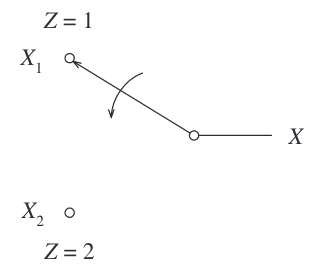 The schematic for (Concavity of Entropy)
According to 2 RVs information diagram where all measures on atoms are Shannon’s measure, we have:
\[\begin{align} H(X)=&\mu^*(\tilde{X})\geq \mu^*(\tilde{X}-\tilde{Z})=H(X\vert Z)\\ =&Pr\{Z=1\}H(X\vert Z=1)+Pr\{Z=2\}H(X\vert Z=2)\\ =&\lambda H(X_1)+(1-\lambda)H(X_2) \end{align}\]which shows that \(H(X)\) is the concave functional of \(p(X)\).
Lemma 4.2.
(Convexity of Mutual Information):
Let \((X,Y)\sim p(x,y)\), then \(I(X;Y)\) is a convex functional of \(p(y\vert x)\) and a concave functional of \(p(x)\).
Proof.
Similar to the proof of (Concavity of Entropy).Omitted
Lemma 4.3.
(Imperfect Secrecy Theorem):
Let \(X\) be the plain text, \(Y\) be the cipher text, and \(Z\) be the key in a secret key crypto system. Since \(X\) can be recovered from \(Y\) and \(Z\), we have \(H(X\vert Y,Z) = 0\). This constraint implies \(I(X;Y)\geq H(X)-H(Z)\).
Especially when a perfectly security is requires, i.e., \(I(X;Y)=0\), \(H(Z)\) is at least \(H(X)\).
(Note: The quantity of \(I(X;Y)\) are often used to measure the security level of the crypto system. We want to make it small so that eavesdroppers cannot get too much information about \(X\) by observing \(Y\). So \(H(Z)\) (called the length of secret key) should be sufficiently large.)
Lemma 4.4.
When \(X\to Y\to Z\to T\to U\) forms a Markov chain, then
\[\begin{align} H(Y)+H(T)=I(Z;X,Y,T,U)+I(X,Y;T,U)+H(Y\vert Z)+H(T\vert Z) \end{align}\]Lattice on RVs
We finish the structure of I-measure and link the Information measures with set theory. The following part of this chapter will link the Shannon’s information measures and McGill’s mutual information with lattice theory. We shall confine ourselves to the case of discrete finite alphabets (called admissible distribution) in consistent with I-measure, while the continuous case is treated with a slight modification.
Let \(X^n=(X_1,\cdots, X_n)\) be \(n\in\mathbb{N}\)-dimension RVs, we have the marginal distribution:
\[\begin{align} \forall \mathcal{D}\subseteq [n],\quad Pr\{\forall i\in \mathcal{D}, X_i=x_i\}=\sum_{j\in [n]-\mathcal{D}}\sum_{x_j\in \mathcal{X}_j}p(x_1,\cdots,x_n) \end{align}\]Definition 5.1.
(Boolean Lattice of RVs):
A \(n\)-dimension Boolean \(\mathbf{X}\) lattice of RVs with join \(\vee\) and meet \(\wedge\) is formed of all subsets of \(\{X_1,\cdots, X_n\}\) with regard to the set inclusion:
(Note: So equivalently, \(\mathbf{X}\) may be regarded as the set of all marginal variable vectors of \(X_{[n]}\).)
Example 5.1.
(Variable Vectors in Boolean Lattice \(\mathbf{X}\)):
- (0-dimensional): \(\emptyset\), which is regarded as a RV taking a constant value with probability 1.
- (1-dimensional): Singletons \(\{X_a\}\)’s, which is called the atoms of the lattice \(\mathbf{X}\).
- (Maximum element): \(E=X_{[n]}\).
Definition 5.2.
(Properties of Boolean Lattice):
- (Complement): Let \(\alpha\in \mathbf{X}\), then there exists the unique \(\bar{\alpha}\in \mathbf{X}\), called the complement of \(\alpha\), such that
- (Partial order): \(\forall \alpha, \beta\in \mathbf{X}, \alpha\leq \beta \iff \alpha \wedge \beta =\alpha\iff \alpha \vee \beta =\beta\).
- (Rank): \(\forall \alpha\in\mathbf{X},r(\alpha)=\vert \alpha\vert\).
- (Interval): \(\forall \alpha,\beta\in \mathbf{X}, \alpha\leq \beta, [\alpha,\beta]=\{\gamma\in\mathbf{X}: \alpha\leq \gamma \leq \beta \}\), which is also called a \((r(\beta)-r(\alpha))\)(length of interval)-dimensional sublattice of \(\mathbf{X}\).
Definition 5.3.
(Functions Defined on Partial Ordered Set):
Let \((\mathbf{L},\leq)\) be a partial ordered set with minimum element \(\emptyset\) and \(f:\mathbf{L}\to \mathbb{R}\) be a function. The difference of \(f\) is defined by:
where the \(\mu: \mathbf{L}^2\to \mathbb{R}\) is called the Mobius function defined by:
\[\begin{align} \sum_{\gamma\leq \beta \leq \alpha}\mu(\gamma,\beta)=\delta_{\gamma,\alpha},\qquad \mu(\alpha,\beta)=0,\forall \alpha <\beta \end{align}\]The sum of \(f\) is defined by:
\[\begin{align} \sum f(\alpha)=\sum_{\emptyset \leq \beta\leq \alpha}f(\beta) \end{align}\]Lemma 5.1.
\[\begin{align} \sum_{\emptyset\leq \beta\leq \alpha}f(\beta)=f(\alpha) \end{align}\]Proof.
\[\begin{align} \sum_{\emptyset\leq \beta\leq \alpha}f(\beta)=& \sum_{\emptyset\leq \beta\leq \alpha}\sum_{\emptyset\leq \gamma\leq \beta}\mu(\gamma, \beta)f(\gamma)=\sum_{\emptyset\leq \gamma\leq \alpha}\sum_{\gamma\leq \beta \leq \alpha}\mu(\gamma,\beta)f(\gamma)\\ =&\sum_{\emptyset\leq \beta\leq \alpha}f(\gamma)\sum_{\emptyset\leq \gamma\leq \beta}\mu(\gamma, \beta)=\sum_{\emptyset\leq \beta\leq \alpha}f(\gamma)\delta_{\gamma,\alpha}=f(\alpha) \end{align}\]Lemma 5.2.
The Mobius function \(\mu(\beta,\alpha)\) is given by:
\[\begin{align} \mu(\beta,\alpha)=\begin{cases} (-1)^{r(\alpha)-r(\beta)},\quad & \text{ for } \beta\leq\alpha,\\0,&\text{ otherwise.} \end{cases} \end{align}\]Proof.
By induction.
We can validate that entropy is a function defined on a Boolean Lattice of RVs \(\mathbf{X}\) with
\[\begin{align} \forall \alpha\in \mathbf{X}, H(\alpha)=-\sum_{(x_{a_1},\cdots, x_{a_n})\in\alpha}Pr\{X_{a_1}=x_{a_1},\cdots, X_{a_n}=x_{a_n}\}\log Pr\{X_{a_1}=x_{a_1},\cdots, X_{a_n}=x_{a_n}\} \end{align}\]where \(\alpha=\mathcal{X}_{a_1}\times\cdots\times\mathcal{X}_{a_k}\) with a particular value \(H(\emptyset )=0\). Then the difference of \(H\) is:
\[\begin{align} \Delta H(\alpha)=\sum_{\emptyset\leq \beta\leq \alpha}(-1)^{r(\alpha)-r(\beta)}H(\beta) \end{align}\]Alternatively, by considering oprator \(\Delta_{\delta}\) on the interval \([\delta,E]\) instead of \(\Delta:[\emptyset, E]\),
\[\begin{align} \Delta_{\delta} H(\alpha)=\sum_{\delta\leq \beta\leq \alpha}(-1)^{r(\alpha)-r(\beta)}H(\beta) \end{align}\]Lemma 5.3.
(McGill’s Mutual information):
\[\begin{align} I(X_{\alpha})=&-1^{r(\alpha)-1}\Delta H(\alpha)\\ I(X_{a_1},;\cdots;X_{a_l}\vert X_{b_1},\cdots,X_{b_m})=&-1^{r(\alpha)-r(\delta)-1}\Delta_{\delta} H(\alpha) \end{align}\]
where \(\alpha \wedge \bar{\delta}=X_{a_1}\vee\cdots,\vee X_{a_l}\) and \(\delta=X_{b_1}\vee\cdots\vee X_{b_m}\).
In the following context of this passage, if it is distinct, we use \(I(X_{\alpha}\vert X_{\beta})\) to denote the mutual information between RVs in \(X_{\alpha}\) conditioning on RVs in \(X_{\beta}\) for convenience.
Example 5.2.
- \(\alpha=X_1, \delta=\emptyset\): Entropy \(H(X_1)\)
- \(\alpha=X_1\vee X_2, \delta=\emptyset\): Shannon’s Mutual Information \(I(X_1;X_2)\)
- \(\alpha=X_1\vee X_2\vee X_3, \delta=\emptyset\): McGill’s Mutual Information \(I(X_1;X_2;X_3)\)
- \(\alpha=X_1\vee X_2, \delta=X_2\): Conditional Entropy \(H(X_1\vert X_2)\).
- \(\alpha=X_1\vee X_2\vee X_3, \delta=X_4\): McGill’s Conditional Mutual Information \(I(X_1;X_2;X_3\vert X_4)\)
We see from (McGill’s Mutual information in Lattice) that all Shannon’s information measures as well as the McGill’s mutual information are in one-to-one correspondence with the intervals of \(\mathbf{X}\). To simplify, we define a function to denote all possible information measures:
Definition 5.4.
(Lattice-theoretic Entropy Function):
Let \(\mathbf{X}_2\) be the set of all intervals of \(\mathbf{X}\), we construct an entropy function \(H: \mathbf{X}_2\to\mathbb{R}\) that for all \(B\in\mathbf{X}_2\) that \(B=[\delta,\alpha]\),
Lemma 5.4.
- The lattice-theoretic entropy function \(H: \mathbf{X}_2\to\mathbb{R}\) is equivalent to the entropy function of \(\mathbf{X}\).
- The number of all different \(\Delta H(\alpha)\)’s, excluding the trivial one \(\Delta H(\emptyset)=0\), is \(2^n-1\), which is the same as that of all different \(H(\alpha)\)’s excluding the trivial one. The result corresponds to [Lemma Number of Atoms].
- the number of all different \(H(B)\)’s is larger than \(2^n-1\) when \(n\geq 2\). Therefore, the \(H(B)\)’s are not all independent.